估计高斯混合模型参数的三种方式
| 博客 | cnblogs |
|---|---|
| 作者 | szcf-weiya |
| 发布 | 2018-01-26 |
| 更新 | 2018-02-04 |
对于如下的两类别的高斯混合模型
参数为$\theta = (\pi, \mu_1,\mu_2,\sigma_1,\sigma_2)$。至今,我了解到有三种方式来估计这五个参数。这三种方式分别为梯度下降法、EM算法和Gibbs采样,而且这三种算法并非毫不相关。EM算法其实是简化梯度下降法中对于对数似然的计算,而Gibbs采样跟EM算法区别在于前者采样后者求最大值。
梯度下降法
思想其实很简单,就是极大似然法,但是解析形式不好确定,好在我们可以通过梯度下降来实现,而且现在有很方便的深度学习框架(如tensorflow)可以实现梯度下降,从而估计参数。下面用一个实际的例子(取自为什么统计学家也应该学学 TensorFlow)来展示梯度下降这一过程
import numpy as np
import matplotlib.pyplot as plt

np.random.seed(123)
# Parameters
p1 = 0.3
p2 = 0.7
mu1 = 0.0
mu2 = 5.0
sigma1 = 1.0
sigma2 = 1.5

# Simulate data
N = 1000
x = np.zeros(N)
ind = np.random.binomial(1, p1, N).astype('bool_')
n1 = ind.sum()
x[ind] = np.random.normal(mu1, sigma1, n1)
x[np.logical_not(ind)] = np.random.normal(mu2, sigma2, N - n1)

# Histogram
#plt.hist(x, bins=30)
#plt.show()

# #############

import tensorflow as tf
import tensorflow.contrib.distributions as ds

# Define data
t_x = tf.placeholder(tf.float32)

# Define parameters
t_p1_ = tf.Variable(0.0, dtype=tf.float32)
t_p1 = tf.nn.softplus(t_p1_)
t_mu1 = tf.Variable(0.0, dtype=tf.float32)
t_mu2 = tf.Variable(1.0, dtype=tf.float32)
t_sigma1_ = tf.Variable(1.0, dtype=tf.float32)
t_sigma1 = tf.nn.softplus(t_sigma1_)
t_sigma2_ = tf.Variable(1.0, dtype=tf.float32)
t_sigma2 = tf.nn.softplus(t_sigma2_)

# Define model and objective function
t_gm = ds.Mixture(
    cat=ds.Categorical(probs=[t_p1, 1.0 - t_p1]),
    components=[
        ds.Normal(t_mu1, t_sigma1),
        ds.Normal(t_mu2, t_sigma2),
    ]
)
t_ll = tf.reduce_mean(t_gm.log_prob(t_x))

# Optimization
optimizer = tf.train.GradientDescentOptimizer(0.5)
train = optimizer.minimize(-t_ll)

# Run
sess = tf.Session()
init = tf.global_variables_initializer()
sess.run(init)
for _ in range(500):
    sess.run(train, {t_x: x})

print('Estimated values:', sess.run([t_p1, t_mu1, t_mu2, t_sigma1, t_sigma2]))
print('True values:', [p1, mu1, mu2, sigma1, sigma2])
EM算法
这一部分在我的ESL-CN翻译项目的8.5 EM算法一节中有详细介绍。具体算法如下:
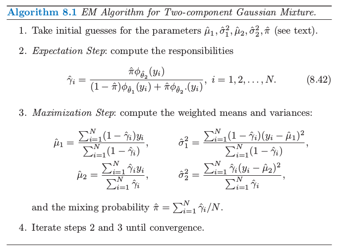
R语言代码如下(也可以在ESL-CN项目中找到):
## EM Algorithm for Two-component Gaussian Mixture
##
## author: weiya
## date: 2017-07-19

## construct the data in figure 8.5
y = c(-0.39, 0.12, 0.94, 1.67, 1.76, 2.44, 3.72, 4.28, 4.92, 5.53,
      0.06, 0.48, 1.01, 1.68, 1.80, 3.25, 4.12, 4.60, 5.28, 6.22)

## left panel of figure 8.5
hist(y, breaks = 12, freq = FALSE, col = "red", ylim = c(0, 1))

## right panel of figure 8.5
plot(density(y), ylim = c(0, 1), col = "red")
rug(y)


fnorm <- function(x, mu, sigma)
{
  return(1/(sqrt(2*pi)*sigma)*exp(-0.5*(x-mu)^2/sigma))
}

IterEM <- function(mu1, mu2, sigma1, sigma2, pi0, eps)
{
  cat('Start EM...\n')
  cat(paste0('pi = ', pi0, '\n'))
  iters = 0
  ll = c()
  while(TRUE)
  {
    ## Expectation step: compute the responsibilities
    ## calculate the delta's expectation
    gamma = sapply(y, function(x) pi0*fnorm(x, mu2, sigma2)/((1-pi0)*fnorm(x, mu1, sigma1) + pi0*fnorm(x, mu2, sigma2)))
    ll = c(ll, sum((1-gamma)*log(fnorm(y,mu1,sigma1))+gamma*log(fnorm(y, mu2, sigma2))+(1-gamma)*log(1-pi0)+gamma*log(pi0)))
    ## Maximization Step: compute the weighted means and variances
    mu1.new = sum((1-gamma)*y)/sum(1-gamma)
    mu2.new = sum(gamma*y)/sum(gamma)
    sigma1.new = sqrt(sum((1-gamma)*(y-mu1.new)^2)/sum(1-gamma))
    sigma2.new = sqrt(sum((gamma)*(y-mu2.new)^2)/sum(gamma))
    pi0.new = sum(gamma)/length(y)
    cat(paste0('pi = ', pi0.new, '\n'))
    if (abs(pi0.new-pi)< eps || iters > 50)
    {
      cat('Finish!\n')
      cat(paste0('mu1 = ', mu1.new, '\n',
                 'mu2 = ', mu2.new, '\n',
                 'sigma1^2 = ', sigma1.new^2, '\n',
                 'sigma2^2 = ', sigma2.new^2))
      break
    }
    mu1 = mu1.new
    mu2 = mu2.new
    sigma1 = sigma1.new
    sigma2 = sigma2.new
    pi0 = pi0.new
    iters = iters + 1
  }
  return(ll)
}
## take initial guesses for the parameters
mu1 = 4.5; sigma1 = 1
mu2 = 1; sigma2 = 1
pi0 = 0.1
eps = 0.01
ll = IterEM(mu1, mu2, sigma1, sigma2, pi0, eps)

## Figure 8.6
plot(1:length(ll), ll, xlab = 'iterations', ylab = 'Log-likelihood', 'o')
Gibbs采样
这一部分在我的ESL-CN翻译项目的8.6 MCMC向后采样一节中有详细介绍。具体算法如下:

R语言代码如下(也可以在ESL-CN项目中找到):
## Gibbs sampling for mixtures
## based on the algorithm 8.4 of ESL
##
## Author: weiya
## Date: 2017.09.12

## data in figure 8.5
y = c(-0.39, 0.12, 0.94, 1.67, 1.76, 2.44, 3.72, 4.28, 4.92, 5.53,
      0.06, 0.48, 1.01, 1.68, 1.80, 3.25, 4.12, 4.60, 5.28, 6.22)

## initial values
mu1 = 4
mu2 = 1
sigma1 = 0.93
sigma2 = 0.88
N = length(y)
t = 0
mu1.h = mu1
mu2.h = mu2
Delta = rep(c(0, 1), each = N/2)
pi0 = sum(Delta)/N
pi0.h = pi0
while(TRUE)
{
  t = t + 1
  gamma = sapply(1:N, function(i) pi0*dnorm(y[i], mu2, sigma2)/((1-pi0)*dnorm(y[i], mu1, sigma1)+pi0*dnorm(y[i], mu2, sigma2)))
  ## sample Delta
  r = runif(N)
  Delta[gamma < r] = 0
  Delta[gamma >= r] = 1
  pi0 = sum(Delta)/N
  ## re-calculate mu1 and mu2
  mu1 = sum((1-Delta)*y)/(sum(1-Delta)+1e-10)
  mu2 = sum(Delta*y)/(sum(Delta)+1e-10)
  ## print info
  cat("t = ", t, "\n")
  for (i in 1:N)
    cat(Delta[i], " ")
  cat("\n")
  cat("mu1 = ", mu1, " mu2 = ", mu2, "pi0 = ",pi0, "\n")

  ## generate mu1 and mu2
  mu1 = rnorm(1, mu1, sigma1)
  mu2 = rnorm(1, mu2, sigma2)
  mu1.h = c(mu1.h, mu1)
  mu2.h = c(mu2.h, mu2)
  pi0.h = c(pi0.h, pi0)
  if (t > 200)
    break
}

## res
## sometimes good, while sometimes bad.
## In addition, sometimes mu1 and mu2 are inverted.