Resampling Methods
weiya
April 28, 2017 (update: February 27, 2019)
Resampling Methods
Resampling methods involve repeatedly drawing samples from a training set and refitting a model of interest on each sample in order to obtain additional information about the fitted model.
estimate the variability of a linear regression fit:
- repeatedly draw different samples from the training data
- fit a linear regression to each new sample
- examine the extent to which the resulting fits differ
two of the most commonly used resampling methods
- cross-validation
- bootstrap
Cross-Validation
The Validation Set Approach
It involves randomly dividing the available set of observations into two parts, a training set and a validation set or hold-out set.
- LOOCV
- \(k\)-fold CV
Remark:
- When we examine real data, we do not know the true test MSE, and so it is difficult to determine the accuracy of the cross-validation estimate
- If we examine simulated data, then we can compute the true test MSE, and can thereby evaluate the accuracy of our cross-validation results.
our goal
determine how well a given statistical learning procedure can be expected to perform on independent data; in this case, the actual estimate of the test MSE is of interest. we are interested only in the location of the minimum point in the estimated test MSE curve.
Bootstrap
can be used to estimate the standard errors of the coefficients from a linear regression fit
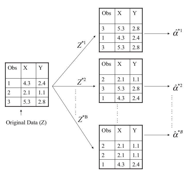
Example
two financial assets that yield returns of \(X\) and \(Y\)
\(\alpha X+(1-\alpha)Y\), where
\[ \alpha = \frac{\sigma_Y^2-\sigma_{XY}}{\sigma_X^2+\sigma^2_Y-2\sigma_{XY}} \]
we want to estimate
\[ \hat\alpha = \frac{\hat\sigma_Y^2-\hat\sigma_{XY}}{\hat\sigma_X^2+\hat\sigma^2_Y-2\hat\sigma_{XY}} \]
\[ SE_B(\hat\alpha)=\sqrt{\frac{1}{B-1}\sum\limits_{r=1}^B(\alpha^{*r}-\frac{1}{B}\sum\limits_{r'=1}^B\hat\alpha^{*r'})^2} \]
Lab
The Validation Set Approach
library(ISLR)
set.seed(1)
train = sample(392, 196)
attach(Auto)
## The following objects are masked from Auto (pos = 4):
##
## acceleration, cylinders, displacement, horsepower, mpg, name,
## origin, weight, year## linear regression
lm.fit = lm(mpg ~ horsepower, data = Auto, subset = train)
mean((mpg - predict(lm.fit, Auto))[-train]^2)## [1] 26.14142## polynomial regression
lm.fit2 = lm(mpg ~ poly(horsepower, 2), data = Auto, subset = train)
mean((mpg-predict(lm.fit2, Auto))[-train]^2)## [1] 19.82259## cubic regression
lm.fit3 = lm(mpg ~ poly(horsepower, 3), data = Auto, subset = train)
mean((mpg-predict(lm.fit3, Auto))[-train]^2)## [1] 19.78252LOOCV
library(boot)
glm.fit = glm(mpg ~ horsepower, data = Auto)
cv.err = cv.glm(Auto, glm.fit)
cv.err$delta
## [1] 24.23151 24.23114It would return a vector of length two. The first component is the raw cross-validation estimate of prediction error. The second component is the adjusted cross-validation estimate. The adjustment is designed to compensate for the bias introduced by not using leave-one-out cross-validation.
cv.error = rep(0, 5)
for (i in 1:5){
  glm.fit = glm(mpg ~ poly(horsepower, i), data = Auto)
  cv.error[i] = cv.glm(Auto, glm.fit)$delta[1]
}
cv.error
## [1] 24.23151 19.24821 19.33498 19.42443 19.03321\(k\)-fold CV
set.seed(17)
cv.error.10 = rep(0, 10)
for (i in 1:10){
  glm.fit = glm(mpg~poly(horsepower, i), data = Auto)
  cv.error.10[i] = cv.glm(Auto, glm.fit, K = 10)$delta[1]
}
cv.error.10
## [1] 24.20520 19.18924 19.30662 19.33799 18.87911 19.02103 18.89609
## [8] 19.71201 18.95140 19.50196Bootstrap
Estimating the Accuracy of a Statistic of Interest
Two steps:
- create a function that computes the statistic of interest
- use the
boot()function, which is part of the boot library, to perform the bootstrap by repeatedly sampling observations from the data set with replacement.
alpha.fn = function(data, index){
  X = data$X[index]
  Y = data$Y[index]
  return((var(Y)-cov(X,Y))/(var(X)+var(Y)-2*cov(X,Y)))
}
alpha.fn(Portfolio, 1:100)
## [1] 0.5758321set.seed(1)
alpha.fn(Portfolio, sample(100, 100, replace = T))## [1] 0.5963833boot(Portfolio, alpha.fn, R = 1000)##
## ORDINARY NONPARAMETRIC BOOTSTRAP
##
##
## Call:
## boot(data = Portfolio, statistic = alpha.fn, R = 1000)
##
##
## Bootstrap Statistics :
## original bias std. error
## t1* 0.5758321 -7.315422e-05 0.08861826Estimating the Accuracy of a Linear Regression Model
The bootstrap approach can be used to assess the variability of the coefficient estimates and predictions from a statistical learning method.
boot.fn = function(data, index)
  return(coef(lm(mpg~horsepower, data = data, subset = index)))

boot.fn(Auto, 1:392)
## (Intercept) horsepower
## 39.9358610 -0.1578447set.seed(1)
boot.fn(Auto, sample(392, 392, replace = T))## (Intercept) horsepower
## 38.7387134 -0.1481952boot(Auto, boot.fn, 1000)##
## ORDINARY NONPARAMETRIC BOOTSTRAP
##
##
## Call:
## boot(data = Auto, statistic = boot.fn, R = 1000)
##
##
## Bootstrap Statistics :
## original bias std. error
## t1* 39.9358610 0.0296667441 0.860440524
## t2* -0.1578447 -0.0003113047 0.007411218summary(lm(mpg~horsepower, data = Auto))$coef## Estimate Std. Error t value Pr(>|t|)
## (Intercept) 39.9358610 0.717498656 55.65984 1.220362e-187
## horsepower -0.1578447 0.006445501 -24.48914 7.031989e-81- although the formula for the standard errors do not rely on the linear model being correct, the estimate for \(\sigma^2\) does.
- the standard formulas assume (somewhat unrealistically) that the \(x_i\) are fixed, and all the variability comes from the variation in the errors \(\epsilon_i\). The bootstrap approach does not rely on any of these assumptions
boot.fn = function(data, index)
coef(lm(mpg~horsepower+I(horsepower^2), data = data, subset = index))
set.seed(1)
boot(Auto, boot.fn, 1000)
##
## ORDINARY NONPARAMETRIC BOOTSTRAP
##
##
## Call:
## boot(data = Auto, statistic = boot.fn, R = 1000)
##
##
## Bootstrap Statistics :
## original bias std. error
## t1* 56.900099702 6.098115e-03 2.0944855842
## t2* -0.466189630 -1.777108e-04 0.0334123802
## t3* 0.001230536 1.324315e-06 0.0001208339summary(lm(mpg~horsepower+I(horsepower^2), data = Auto))$coef## Estimate Std. Error t value Pr(>|t|)
## (Intercept) 56.900099702 1.8004268063 31.60367 1.740911e-109
## horsepower -0.466189630 0.0311246171 -14.97816 2.289429e-40
## I(horsepower^2) 0.001230536 0.0001220759 10.08009 2.196340e-21Copyright © 2016-2019 weiya